Demo example: Analysis

This example is the continuation of the previous example: filling gaps and missing observations. This example serves as an introduction to the Analysis module.

import metobs_toolkit

your_dataset = metobs_toolkit.Dataset()
your_dataset.update_settings(
    input_data_file=metobs_toolkit.demo_datafile, # path to the data file
    input_metadata_file=metobs_toolkit.demo_metadatafile,
    template_file=metobs_toolkit.demo_template,
)
#Update Gap definition
your_dataset.update_qc_settings(gapsize_in_records = 20)

#Import the data
your_dataset.import_data_from_file()

#Coarsen to 15-minutes frequencies
your_dataset.coarsen_time_resolution(freq='15T')

#Apply default quality control
your_dataset.apply_quality_control(obstype='temp') #we use the default settings in this example

#Interpret the outliers as missing observations and gaps.
your_dataset.update_gaps_and_missing_from_outliers(obstype='temp',
                                                   n_gapsize=None)

#Fill missing observations (using default settings)
your_dataset.fill_missing_obs_linear(obstype='temp')

#Fill gaps with linear interpolation.
your_dataset.fill_gaps_linear(obstype='temp')

		temp	temp_final_label
name	datetime
vlinder01	2022-09-02 15:30:00+00:00	26.453659	gap_interpolation
	2022-09-02 15:45:00+00:00	26.207317	gap_interpolation
	2022-09-02 16:00:00+00:00	25.960976	gap_interpolation
	2022-09-02 16:15:00+00:00	25.714634	gap_interpolation
	2022-09-02 16:30:00+00:00	25.468293	gap_interpolation
...	...	...	...
vlinder28	2022-09-15 07:00:00+00:00	14.114815	gap_interpolation
	2022-09-15 07:15:00+00:00	14.251852	gap_interpolation
	2022-09-15 07:30:00+00:00	14.388889	gap_interpolation
	2022-09-15 07:45:00+00:00	14.525926	gap_interpolation
	2022-09-15 08:00:00+00:00	14.662963	gap_interpolation

5111 rows × 2 columns

Creating an Analysis

The built-in analysis functionality is centered around the Analysis class. First, create an Analysis object using the get_analysis() method.

analysis = your_dataset.get_analysis(add_gapfilled_values=True)
analysis

Analysis instance containing:
     *28 stations
     *['humidity', 'precip', 'precip_sum', 'pressure', 'pressure_at_sea_level', 'radiation_temp', 'temp', 'wind_direction', 'wind_gust', 'wind_speed'] observation types
     *38820 observation records
     *Coordinates are available for all stations.

     *records range: 2022-09-01 00:00:00+00:00 --> 2022-09-15 23:45:00+00:00 (total duration:  14 days 23:45:00)     *Coordinates are available for all stations.

Analysis methods

An overview of the available analysis methods can be seen in the documentation of the Analysis class. The relevant methods depend on your data and your interests. As an example, a demonstration of the filter and diurnal cycle of the demo data.

Filtering data

It is common to filter your data according to specific meteorological phenomena or periods in time. To do this you can use the apply_filter() method.

#filter to non-windy afternoons in the Autumn.
subset = analysis.apply_filter('wind_speed <= 2.5 & season=="autumn" & hour > 12 & hour < 20')

subset.df

		humidity	precip	precip_sum	pressure	pressure_at_sea_level	radiation_temp	temp	wind_direction	wind_gust	wind_speed
name	datetime
vlinder01	2022-09-01 18:00:00+00:00	47.0	0.0	0.0	101453.0	101717.0	NaN	22.9	45.0	4.8	1.8
	2022-09-01 18:15:00+00:00	48.0	0.0	0.0	101448.0	101712.0	NaN	22.4	45.0	4.8	1.7
	2022-09-01 18:30:00+00:00	50.0	0.0	0.0	101461.0	101725.0	NaN	21.8	45.0	3.2	0.6
	2022-09-01 18:45:00+00:00	55.0	0.0	0.0	101468.0	101733.0	NaN	20.3	45.0	0.0	0.0
	2022-09-01 19:00:00+00:00	58.0	0.0	0.0	101460.0	101726.0	NaN	18.8	45.0	0.0	0.0
...	...	...	...	...	...	...	...	...	...	...	...
vlinder28	2022-09-15 18:45:00+00:00	76.0	0.0	17.8	101314.0	101266.0	NaN	15.7	15.0	8.1	0.8
	2022-09-15 19:00:00+00:00	76.0	0.0	17.8	101320.0	101272.0	NaN	15.5	15.0	4.8	0.6
	2022-09-15 19:15:00+00:00	77.0	0.0	17.8	101325.0	101277.0	NaN	15.3	5.0	0.0	0.0
	2022-09-15 19:30:00+00:00	78.0	0.0	17.8	101339.0	101291.0	NaN	15.1	65.0	4.8	0.9
	2022-09-15 19:45:00+00:00	79.0	0.0	17.8	101343.0	101295.0	NaN	15.0	65.0	0.0	0.0

6347 rows × 10 columns

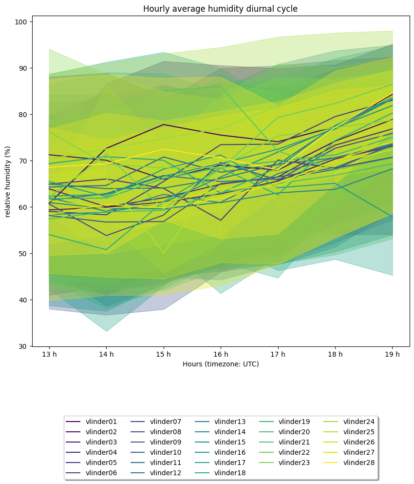
Diurnal cycle

To make a diurnal cycle plot of your Analysis use the get_diurnal_statistics() method:

dirunal_statistics = subset.get_diurnal_statistics(colorby='name',
                                                   obstype='humidity',
                                                   plot=True,
                                                   errorbands=True,
                                                  )
#Note that in this example statistics are computed for a short period and only for the non-windy autumn afternoons.

Analysis exercise

For a more detailed reference you can use this Analysis exercise, which was created in the context of the COST FAIRNESS summer school 2023 in Ghent.